
H2O + AWS + purrr (Part II)
This is the second installment in a three part series on integrating H2O, AWS and p(f)urrr. In Part II, I will showcase how we can combine purrr and h2o to train and stack ML models. In the first post we looked at starting up an AMI on AWS which acts as the infrastructure upon which we will model.
Part one of the post can be found here
The packages we will use in this post:
library(tidyverse)library(h2oEnsemble)library(caret)library(mlbench)
Using purrr to train H2O models
In this post I will be using the r3.4xlarge machine we started up in Part I of this series. The code below starts up a H2O instance that uses all available cores and limits the instance’s memory to 100GB.
h2o.init(nthreads = -1, max_mem_size = '100g')
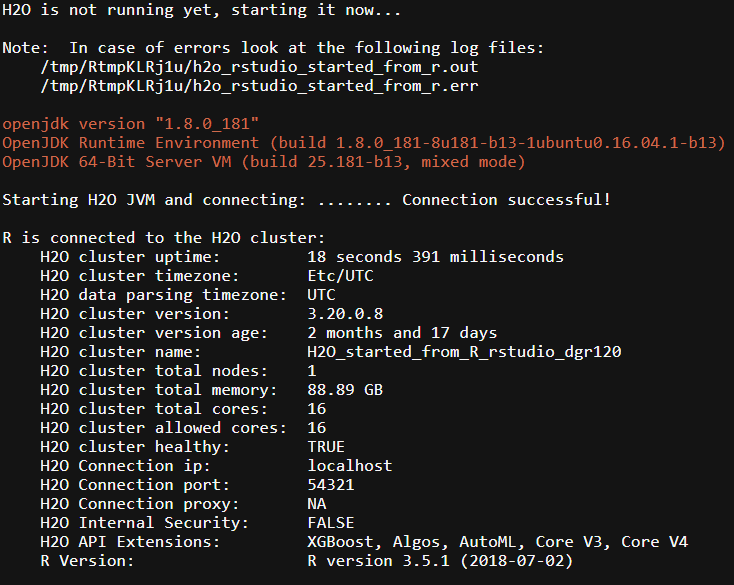
We can see that once the server is up, we have 88.89 GB RAM and 16 Cores available. Also take note of the very handy logging file: /tmp/RtmpKLRj1u/h2o_rstudio_started_from_r.out.
We will use the Higgs data to experiment on:
Using simulated data with features characterizing events detected by ATLAS, your task is to classify events into “tau decay of a Higgs boson” versus “background.”
As per all machine learning application, we need to split our data. We will use the h2o.splitFrame function to split the data into training, validation and test sets. What is very important to notice in the function is the destination_frame parameter as the datasets are being transformed to .hex format which is the required format for the H2O server.
train <- read_csv("https://s3.amazonaws.com/erin-data/higgs/higgs_train_5k.csv")
test <- read_csv("https://s3.amazonaws.com/erin-data/higgs/higgs_test_5k.csv")

higgs <- rbind(train, test) %>%
  mutate(response = as.factor(response))

set.seed(107)
splits <- h2o.splitFrame(
  data = as.h2o(higgs, destination_frame = "higgs.hex"),
  ratios = c(0.6, 0.2),   ## only need to specify 2 fractions, the 3rd is implied
  destination_frames = c("train.hex", "valid.hex", "test.hex"), seed = 1234
)

training <- splits[[1]]
valid <- splits[[2]]
testing <- splits[[3]]
The split frames are now of the correct class H2OFrame. Next we need to specify the outcome and predictor columns:
Y <- 'response'
X <- setdiff(names(training), Y)
To test the basic functionality of H2O, lets train a gbm to predict signal against background noise for the Higgs dataset.
higgs.gbm <- h2o.gbm(y = Y, x = X, training_frame = training, ntrees = 5,
                    max_depth = 3, min_rows = 2, learn_rate = 0.2,
                    distribution = "AUTO")

higgs.gbm
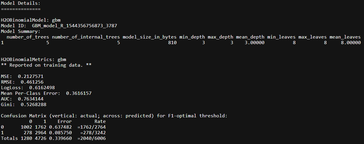
This very basic specification of the model, tuning = {ntrees = 5, max_depth = 3, learning_rate = 0.2}, gives us an AUC of ~77%. Lets see how the model does on the validation set:
h2o.performance(higgs.gbm, valid)
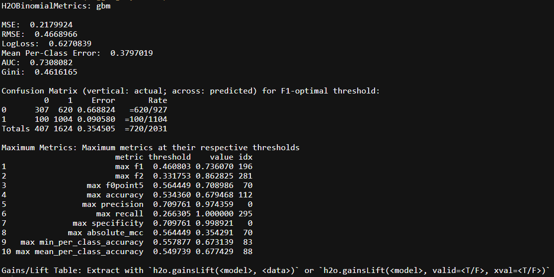
From the validation set we can see that the models don’t perform too differently. It correctly predicts signal vs background with about 35.5% prediction error and AUC of 73%. For the rest of this post we will not be concerning ourselves with models performance, but rather focus on how we can build nice pipelines using H2O and purrr.
Having a basic understanding of the H2O api, lets ramp it up to train multiple models using purrr. The first step is to create a function that contains all the H2O models we want to use in our modeling design. Our wrapper should contain basic parameters: training_frame, validation_frame, nfolds and Y/X variable names.
A very important feature in our new wrapper you should notice is fold_assignment = "Modulo" and keep_cross_validation_predictions = TRUE parameters. We need these as we want to stack the models at a later stage to check if it improves performance1.
h2o.models <- function(df, validation, nfolds, model, Y, X){
  if(model == "gbm"){
    return(h2o.gbm(y = Y, x = X,
                   training_frame = df,
                   validation_frame = validation,
                   distribution = "bernoulli",
                   nfolds = nfolds,
                   fold_assignment = "Modulo",
                   keep_cross_validation_predictions = TRUE))
  }

  if(model == "rf"){
    return(h2o.randomForest(y = Y, x = X,
                            training_frame = df,
                            validation_frame = validation,
                            distribution = "bernoulli",
                            nfolds = nfolds,
                            fold_assignment = "Modulo",
                            keep_cross_validation_predictions = TRUE))
  }

  if(model == "xgboost"){
    return(h2o.xgboost(y = Y, x = X,
                       training_frame = df,
                       validation_frame = validation,
                       distribution = "bernoulli",
                       nfolds = nfolds,
                       fold_assignment = "Modulo",
                       keep_cross_validation_predictions = TRUE))
  }

  if(model == "deeplearning"){
    return(h2o.deeplearning(y = Y, x = X,
                            training_frame = df,
                            validation_frame = validation,
                            distribution = "bernoulli",
                            nfolds = nfolds,
                            fold_assignment = "Modulo",
                            keep_cross_validation_predictions = TRUE))
  }
}
This gives a nice wrapper for use with purrr’s map function. Lets create a tibble that has the necessary layout so we can apply our new function across the dataset. You do not necessarily need to add the training, validation and testing frames into the tibble, but it helps in the long-run, especially if they start differing somehow2. It also helps for auditing the models:
trained_ML <- tibble(Models = c("gbm", "rf", "deeplearning", "xgboost")) %>%
  mutate(
    training = rep(list(training), nrow(.)),
    valid = rep(list(valid), nrow(.))
    )
trained_ML
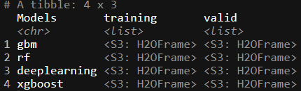
Here we see that we have a special column, `Models’, specifically naming the algorithm assigned to a training and test set.
Lets now use the h2o.models function by training all the different models and evaluating their performance.
trained_ML <- tibble(Models = c("gbm", "rf", "deeplearning", "xgboost")) %>%
  mutate(
    training = rep(list(training), nrow(.)),
    valid = rep(list(valid), nrow(.))
    ) %>%
  # pmap to apply the h2o functional across each row
  mutate(trained_models = pmap(list(training, valid, Models), ~h2o.models(..1, ..2, ..3, nfolds = 5, Y, X))) %>%
  # once trained, predict against the test set with respective model gbm etc
  mutate(predictions = map(trained_models, h2o.predict, testing)) %>%
  # create new column containing in-sample confusionMatrix
  mutate(confusion = map(trained_models, h2o.confusionMatrix)) %>%
  # create new column containing test set performance metrics
  mutate(performance = map2(trained_models, valid, ~h2o.performance(.x, .y)))
trained_ML
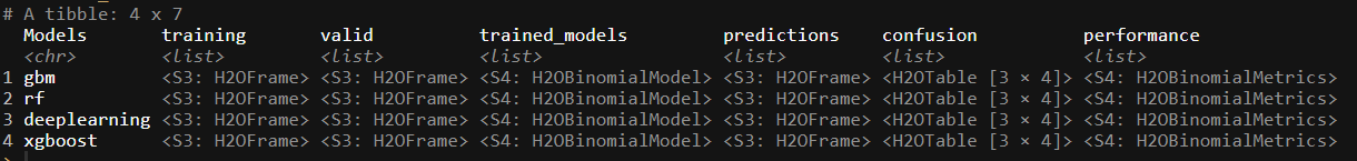
As a last measure, we might not want to have the performance metrics nested in the tibble frame. So to lift the measures out of the performance list, we can build our own function to extract the performance metrics we might need in evaluating each of the model’s performance:
f_perf <- function(performance){
  tibble(errors = tail(performance@metrics$cm$table$Error, 1),
  logloss = performance@metrics$logloss,
  rmse = performance@metrics$RMSE,
  r_sqaured = performance@metrics$r2,
  pr_auc = performance@metrics$pr_auc,
  gini = performance@metrics$Gini)
}

trained_ML <- trained_ML %>%
    bind_cols(map_df(.$performance,  f_perf))
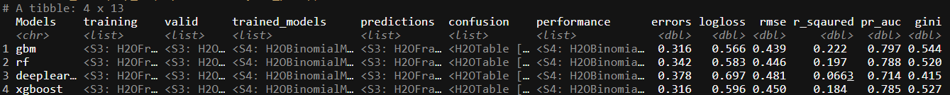
This new tibble gives us a very good idea on which model performs the best, if we base it off the logloss measure of fit: gbm. From here we could build a wrapper around different gbm models and use the same framework to train multiple different types of gbm specified models if we wanted to do so.
The last bit of performance improvement we attempt in any model process is stacking. Model stacking is the idea that using the predictions of the base learners (in our case the rf, gbm etc), and then using a super learner or meta learner that takes as input, the base learners predictions/CV results and runs a model across those results as the final prediction. There are some interesting papers which talk to this idea, one by Leo Breiman3 himself or another one by van der Laan, Polley, and Hubbard 2007 that statistically proves why these Super Learners work.
As my metalearner in this example I will use a glm:
models <- trained_ML %>%
  pull(trained_models)

metalearner <- c("h2o.glm.wrapper")

stack <- h2o.stack(models = models,
          response_frame = training[,Y],
          metalearner = metalearner,
          seed = 1,
          keep_levelone_data = TRUE)

# Compute test set performance:
perf <- h2o.ensemble_performance(stack, newdata = testing)$ensemble

stack_df <- tibble(Models = "stack",
       trained_models = list(stack),
       performance = list(perf)) %>%
  bind_cols(map_df(.$performance,  f_perf))

bind_rows(trained_ML,stack_df)
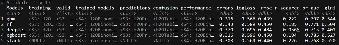
Our stack of the models do not seem to improve the logloss performance measure in this specific case. That being said, we haven’t spent a lot of time trying to tune any of the models.
The last bit of code we need to finish this pipeline is to shutdown the H2O server:
h2o.ls()
h2o.removeAll()
h2o.shutdown()
Conclusion
As you can see, combining the Many-models idea with the engineering of H2O and AWS, gives us a very nice framework with which we can run a crazy amount of experiments at a low cost and within a short time period. In writing this blog, I spent a total of 2 hours and 40 minutes running the models multiple times, getting the stack to work and overall just reading some H2O documentation. While all this was happening our r3.4xlarge - 16 core, 100GB RAM machine was running, resulting in a total cost for this blog at around $0.42, give or take. Which I think isn’t too bad for the resources that we used.
In the last and final part of the series, we will explore how to initialize a H2O AWS server using furrr and a basic script. This means that you can essentially write the code on your home setup, use boto3 from python to spin up an EC2 instance, conduct the analysis and only return to your local environment the most important results.