
As part of my studies, I have been exploring models and how they can be used to compartmentalize clusters within text. This comes as I have been knee deep in Julia Silge’s tidytext book1. One of the chapters (ch 6) in the book introduces the idea of Topic Models and how Latent Dirichlet allocation (LDA) is a very good tool in order to create these natural underlying groupings. Further reading into the subject lead me to discover a recent post, yes - by Julia again, on how she uses Structural Topic Models to gain insight into how the models operate using the stories from Sherlock Holmes.
This was the final motivation for me to go and find out for myself how this new class of Structural topic models work and maybe also learn something new about the news that surrounds the crypto market. In this post I will be exploring some of the functions of the stm package created by Molly Roberts, Brandon Stewart and Dustin Tingley by exploring the news released by Coindesk in the market news section. The idea is to gain some insight into what the topics are that are getting published and also, perhaps see if how the topics shift over time in the crypto markets.
Getting the news data
To get the news data, I used Rselenium, a powerful package that helps to simulate a webbrowser that is able to interact with elements in a webpage. Since this post isn’t too fussed on the inner workings of RSelenium, I will only show you the end result of the data collected2. If you are keen to see how one can use RSelenium in online collection tasks, I will be giving a workshop on it at UseR!2018, - so be on the lookout for the tutorial if you are attending the conference.
So start by reading in the news articles and the meta data we have around each article
coindesk <- read_rds("all_articles.rds")
glimpse(coindesk)
## Observations: 610
## Variables: 3
## $ pg_date  <date> 2018-03-04, 2018-03-03, 2018-03-02, 2018-03-02, 2018...
## $ link     <chr> "https://www.coindesk.com/crypto-stars-turn-truth-mac...
## $ articles <chr> "There seems to be an audible buzz.  It's been a long...
Here we can see that the data is organised so that each observation consists out of a Date, link and the actual text of the article collected. This format makes it easy to implement the tidy principles from the tidytext package. Next, we clean up the data by applying a tokenizer (stripping the article into single words) and then removing all uneccesary stopwords
coindesk_tidy <- coindesk %>%
  unnest_tokens(word, articles) %>%
  anti_join(stop_words, by = "word") %>%
  mutate(word = trimws(word)) %>%
  ungroup

coindesk_tidy %>%
    count(word, sort = TRUE)
## # A tibble: 10,820 x 2
##                word     n
##               <chr> <int>
##  1          bitcoin  2163
##  2   cryptocurrency  1116
##  3            price  1013
##  4           market   931
##  5          trading   853
##  6          percent   758
##  7             time   719
##  8         exchange   654
##  9 cryptocurrencies   427
## 10        exchanges   388
## # ... with 10,810 more rows
The top words from all the articles are bitcoin (obvious), crytocurrency, price, market and so forth. Its important to see that there are actual duplicates in the text data, such as crytocurrency and crytocurrencies (the plural). This is a strong case for stemming the words after applying the tokenizer to avoids such occurances. But, we will leave this kind of intensive text pre-processing for another day. To cull some of the most common words, we turn to technique called tf-idf, which stands for term frequency - inverse document frequency. This measures how important all the words in the complete corpus are in explaining single articles. The more often a word occurs in an article, the higher the tf-idf score of that word. On the other hand, if the word is common to all articles, meaning the word has a high frequency in the whole corpus, the lower that word’s tf-idf score will be. So, from above, we keep the top 10% of words based on tf-idf.
word_keep <- coindesk_tidy %>%
    count(link, word, sort = TRUE) %>%
    bind_tf_idf(., word, link, `n`) %>%
    select(word, tf_idf) %>%
    arrange(desc(tf_idf)) %>%
    filter(tf_idf > quantile(tf_idf, 0.9, na.rm = T)) %>% pull(word)
Now we can just straight into Topic Modeling using the stm package and its workhorse function stm. I decide on 20 topics in order to get a wide range of topics. My hope is to see that there are topics that jump out that focusses on specifc coins. The function takes its input as a document-term matrix. We can also use the output from prepDocuments, but again, lets leave that for now so we can get straight into the analysis. I will use the cast_sparse function from tidytext to coerce the data into a nice sparse matrix.
coindesk_dfm <- coindesk_tidy %>%
    count(link, word, sort = TRUE) %>%
    filter(word %in% word_keep) %>%
     cast_sparse(link, word, n)

topic_model <- stm(coindesk_dfm, K = 20, emtol = 1e-05,
                   verbose = F, init.type = "Spectral")
We now use the broom::tidy method to help us get the model into a tidy data.frame. Once this is done, we can analise the per-topic-per-word distribution. This can help identify which words are most prominent within a specific topic. This measure is also known as the $\beta$-measure
td_beta <- tidy(topic_model)

td_beta %>%
    group_by(topic) %>%
    top_n(10, beta) %>%
    ungroup() %>%
    mutate(topic = paste0("Topic ", topic),
           term = reorder_within(term, beta, topic)) %>%
    ggplot(aes(term, beta, fill = as.factor(topic))) +
    geom_col(alpha = 0.8, show.legend = FALSE) +
    facet_wrap(~ topic, scales = "free_y") +
    coord_flip() +
    scale_x_reordered() +
    labs(x = NULL, y = expression(beta),
         title = "Highest word probabilities for each topic",
         subtitle = "Different words are associated with different topics")
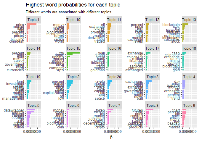
Topic 15 seems to be mostly about Ripple (XRP), while topic 12⁄18 focusses more on when the split happened last year when Bitcoin Gold emerged. We also see that topic 17 isolated the hacks that have occured in the last year. I am also quite suprised that the model was succesful in isolating the launch of the futures market in topics 8 and 11. It also seemed to hint that topic 3 relates to all Asian market activity.
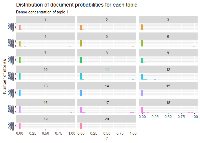
One aspect that we do notice is the high concentration of words such as bitcoin and cryptocurrency. It is this wise to maybe check if stemming and a harsher culling of common words improve the isolation. The need to implement these kind of measures are also evident when we investigate $\gamma$, per-document-per-topic probabilities.
td_gamma <- tidy(topic_model, matrix = "gamma",
                 document_names = rownames(coindesk_dfm))

ggplot(td_gamma, aes(gamma, fill = as.factor(topic))) +
  geom_histogram(alpha = 0.8, show.legend = FALSE) +
  facet_wrap(~ topic, ncol = 3) +
  labs(title = "Distribution of document probabilities for each topic",
       subtitle = "Dense concentration of topic 1",
       y = "Number of stories", x = expression(gamma))
## `stat_bin()` using `bins = 30`. Pick better value with `binwidth`.
Having conducted the analysis using stm, the one frustrating facet of the package is its inability to play nice with the tidyverse in its more niche functions. The ones that I found the most frustrating was the searchK and process functions that I wanted to use. Having processed my data in a tidy fashion early on. I could not use the same object to conduct a cross-validation analysis in order to get an idea of appropriate topics or rely on the effective cleaning procedures the package has.
So, due to this, here is a workflow I propose you use if you want to use the processing and searchK functions in a tidy(ish) fashion.
The initial part aims to process the text data. For this I will use the textProcessor and prepDocuments functions from the stm package. These functions spit out list objects that are quite hard to work with. But that seeing as the searchK function needs a certain kind of input, we will play by the package’s rules later on. For now, lets build a tidyverse friendly version to clean the text.
The function then goes on to conduct the analysis on which amount of topics would be appropriate to use in the eventual model. I will call this function tidy_prepDocuments. As it stands here, the function is very basic and does not have any error handling. For those who would like to bring this into production I suggest adding pre-checks3.
tidy_prepDocuments <- function(df, doc_name, documents, verbose = F){

  options(stringsAsFactors = F)

  documents_col <- enquo(documents)
  doc_name_col <- enquo(doc_name)

  df <- df %>% filter(!is.na(!!documents_col))

  documents <- df %>% pull(!!documents_col)

  if(!missing(doc_name)){
    doc_names <- df %>% pull(!!doc_name_col)
  } else {
    doc_names <- seq(1, length(documents), 1)
  }

  documents_tp <- textProcessor(documents, metadata = df)

  if(length(documents_tp$docs.removed) != 0){
    doc_names <- doc_names[-documents_tp$docs.removed]
  }

  documents_prepped <- prepDocuments(documents_tp[['documents']],
                                     documents_tp[['vocab']],
                                     documents_tp[['meta']],
                                     verbose = verbose)

  if(length(documents_prepped$docs.removed) != 0){
    doc_names <- doc_names[-documents_prepped$docs.removed] %>% as.list
  } else {
    doc_names <- doc_names %>% as.list
  }

  vocab <- documents_prepped$vocab %>% tibble(words = .) %>%
    mutate(word_nr = row_number())

  documents_prepped$documents %>% map(~.x %>%
                                    t %>%
                                    data.frame %>%
                                    rename(word_nr = X1, count = X2)) %>%
    Map(data.frame, document = doc_names, .) %>%
    reduce(rbind) %>%
    left_join(., vocab, by = "word_nr") %>%
    select(document, words, count) %>%
    tbl_df
}

coindesk_prep <- coindesk %>% tidy_prepDocuments(., link, articles)
## Building corpus...
## Converting to Lower Case...
## Removing punctuation...
## Removing stopwords...
## Removing numbers...
## Stemming...
## Creating Output...
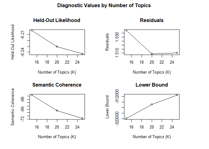
Having done all the hard work on the text data, we can use the same dataset to conduct the grid search that can help to decide on the number of topics we want to use. So lets use the prepped documents objectsin our searchK_tidy function that is nou magrittr friendly:
searchK_tidy <- function(df, document, word, count, K,
                         plot = T, cores = 1, verbose = F){

  document_col <- enquo(document)
  word_col <- enquo(word)
  count_col <- enquo(count)

  vocab <- df %>% select(!!word_col) %>% distinct %>%
    mutate(word_nr = row_number())

  document <- df %>% select(!!document_col, !!word_col, !!count_col) %>%
    left_join(.,vocab) %>%
    rename(., split_col = !!document_col) %>%
    split(., f = .$split_col)

  document <- document %>% map(~.x %>%
                                 select(word_nr, count) %>%
                                 filter(!is.na(word_nr)) %>%
                                 group_by(word_nr) %>%
                                 summarise(count = sum(count)) %>%
                                 as.matrix %>% t)
  vocab <- vocab %>% pull(words)

  sk_results <- searchK(document,
                        vocab, K, init.type = "Spectral",
                        proportion = 0.5, heldout.seed = NULL, M = 10,
                        cores = cores, verbose = verbose)

  if(plot){
    plot.searchK(sk_results)
  }

  sk_results$results %>% tbl_df
}
Lets see these 2 new functions in action and how one would go about using them in an analytical workflow:
coindesk_prep <- coindesk %>% tidy_prepDocuments(., link, articles)
## Building corpus...
## Converting to Lower Case...
## Removing punctuation...
## Removing stopwords...
## Removing numbers...
## Stemming...
## Creating Output...
word_keep <- coindesk_prep %>%
    bind_tf_idf(., words, document, count) %>%
    select(words, tf_idf) %>%
    arrange(desc(tf_idf)) %>%
    filter(tf_idf > quantile(tf_idf, 0.95, na.rm = T)) %>% pull(words)

searched_topics <- coindesk_prep %>%
  filter(words %in% word_keep) %>%
  searchK_tidy(., document, words, count, K = seq(15, 25, 5), cores = 1)
## Joining, by = "words"
coindesk_dfm <- coindesk_prep %>%
     cast_sparse(document, words, count)

topic_model <- stm(coindesk_dfm, K = 20, emtol = 1e-05,
                   verbose = F, init.type = "Spectral")
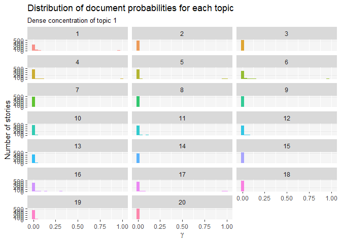
We can see that it didnt change much, we almost got the same distribution of topics and documents. Most of the documents may just be daily price reports. I do think though that given a much larger corpus, it will make a difference:
td_gamma <- tidy(topic_model, matrix = "gamma",
                 document_names = rownames(coindesk_dfm))

ggplot(td_gamma, aes(gamma, fill = as.factor(topic))) +
  geom_histogram(alpha = 0.8, show.legend = FALSE) +
  facet_wrap(~ topic, ncol = 3) +
  labs(title = "Distribution of document probabilities for each topic",
       subtitle = "Dense concentration of topic 1",
       y = "Number of stories", x = expression(gamma))
## `stat_bin()` using `bins = 30`. Pick better value with `binwidth`.
Closing remarks
This post started out by looking to explore the news data generated by Coindesk in an effort to evalaute if certain topics of discussion do emerge.
As part of the anlysis, we wanted to explore the amount of topics we shoud be using in the construction of the model. Having fiddled with the functions that help fascilitate this kind of analysis, we found them frustrating to used in a tidy framework. With this in mind, this post ends of with a small programming experiment where we try and build a suggested framework that is able to process text data using the powerful functions in the stm and also be able to use the searchK function in a tidy manner. The functions are by far not bulletproof in a production sense, but is definately a step in the right direction.
- Which, lets be honest, is a fun and informative read! So highly recommend you have a look at it if you interested in the field of text analysis ^
- Be aware, I only collect this data for research purposes and do not promote people going around randomly scraping whatever website they want ^
- The function is quite lump as well, as it is mostly a thought experiment. Drop a comment if you can build some optimisation into it ^